ASAP Case Study
Updated on 02/17/2022
Source:../../vignettes/003_ASAPCaseStudy.Rmd
003_ASAPCaseStudy.RmdInstall and library packages
remotes::install_github("nmfs-fish-tools/r4MAS")
install.packages("jsonlite")
remotes::install_github("nmfs-general-modeling-tools/nmfspalette")
remotes::install_github("nmfs-fish-tools/fishsad")Read ASAP input file
# Working directory
temp_dir <- tempdir()

# Read ASAP input data
asap_input <- fishsad::asap_simple$input$dat
asap_output <- fishsad::asap_simple$output
Convert ASAP inputs to MAS inputs
# Load r4MAS module
r4mas <- Rcpp::Module("rmas", PACKAGE = "r4MAS")

# Find the path of dynamically-loaded file with extension .so on Linux, .dylib on OS X or .dll on Windows
libs_path <- system.file("libs", package = "r4MAS")
dll_name <- paste("r4MAS", .Platform$dynlib.ext, sep = "")
if (.Platform$OS.type == "windows") {
  dll_path <- file.path(libs_path, .Platform$r_arch, dll_name)
} else {
  dll_path <- file.path(libs_path, dll_name)
}
r4mas <- Rcpp::Module("rmas", dyn.load(dll_path))
# General settings
nyears <- asap_input$n_years

nseasons <- 1

nages <- asap_input$n_ages

ages <- 1:asap_input$n_ages

area1 <- new(r4mas$Area)
area1$name <- "area1"

# Recruitment settings
recruitment <- new(r4mas$BevertonHoltRecruitment)

recruitment$R0$value <- asap_input$SR_scalar_ini / 1000
recruitment$R0$estimated <-
  ifelse(asap_input$phase_SR_scalar < 0, FALSE, TRUE) # TRUE
recruitment$R0$phase <- abs(asap_input$phase_SR_scalar)

recruitment$h$value <- asap_input$steepness_ini
recruitment$h$estimated <-
  ifelse(asap_input$phase_steepness < 0, FALSE, TRUE) # TRUE
recruitment$h$phase <- abs(asap_input$phase_steepness)
recruitment$h$min <- 0.2001
recruitment$h$max <- 1.0

recruitment$sigma_r$value <- sqrt(log((asap_input$recruit_cv[1, ])^2 + 1))
recruitment$sigma_r$estimated <- FALSE
recruitment$sigma_r$min <- 0
recruitment$sigma_r$max <- 3
recruitment$sigma_r$phase <- 2

recruitment$estimate_deviations <-
  ifelse(asap_input$phase_rec_devs < 0, FALSE, TRUE) # TRUE
recruitment$constrained_deviations <- TRUE
recruitment$deviations_min <- -15.0
recruitment$deviations_max <- 15.0
recruitment$deviation_phase <- abs(asap_input$phase_rec_devs)
recruitment$SetDeviations(rnorm(nyears, mean = 0, sd = sqrt(log((asap_input$recruit_cv[1, ])^2 + 1))))
recruitment$use_bias_correction <- FALSE

# Growth settings
growth <- new(r4mas$VonBertalanffyModified)

fleet_num <- asap_input$n_fleets
catch_waa_pointer <- asap_input$WAA_pointers[fleet_num * 2 + 1]
catch_empirical_weight <-
  as.vector(t(asap_input$WAA_mats[[catch_waa_pointer]])) # Total catch

ssb_waa_pointer <- asap_input$WAA_pointers[fleet_num * 2 + 2 + 1]
ssb_empirical_weight <-
  as.vector(t(asap_input$WAA_mats[[ssb_waa_pointer]]))

jan1_waa_pointer <- asap_input$WAA_pointers[fleet_num * 2 + 2 + 2]
jan1_empirical_weight <-
  as.vector(t(asap_input$WAA_mats[[jan1_waa_pointer]]))

survey_num <- 1 # Need to be updated using the code below when MAS can have multiple surveys with different unit
# survey_num <- asap_input$n_indices
survey_empirical_weight <- vector(mode = "list", length = survey_num)
for (i in 1:survey_num) {
  survey_waa_pointer <- asap_input$index_WAA_pointers[i]
  survey_waa <- as.vector(t(asap_input$WAA_mats[[survey_waa_pointer]]))

  if (asap_input$index_units[i] == 1) {
    survey_empirical_weight[[i]] <- survey_waa
  } # Survey unit is biomass

  if (asap_input$index_units[i] == 2) {
    survey_empirical_weight[[i]] <- replicate(nages * nyears, 1.0)
  } # Survey unit is number
}

growth$SetUndifferentiatedCatchWeight(catch_empirical_weight)
growth$SetUndifferentiatedWeightAtSeasonStart(jan1_empirical_weight)
growth$SetUndifferentiatedWeightAtSpawning(ssb_empirical_weight)
growth$SetUndifferentiatedSurveyWeight(survey_empirical_weight[[1]])

# Maturity settings
maturity <- new(r4mas$Maturity)
maturity$values <- asap_input$maturity[1, ]

# Natural mortality settings
natural_mortality <- new(r4mas$NaturalMortality)
natural_mortality$SetValues(asap_input$M[1, ])

# Movement settings
movement <- new(r4mas$Movement)
movement$connectivity_females <- c(0.0)
movement$connectivity_males <- c(0.0)
movement$connectivity_recruits <- c(0.0)

# Initial deviations
initial_deviations <- new(r4mas$InitialDeviations)
initial_deviations$values <- rep(0.0, times = nages)
initial_deviations$estimate <-
  ifelse(asap_input$phase_N1_devs < 0, FALSE, TRUE) # TRUE
initial_deviations$phase <- abs(asap_input$phase_N1_devs)

# Create population
population <- new(r4mas$Population)
for (y in 1:(nyears))
{
  population$AddMovement(movement$id, y)
} # y starts from 0 or 1?

population$AddNaturalMortality(natural_mortality$id, area1$id, "undifferentiated")
population$AddMaturity(maturity$id, area1$id, "undifferentiated")
population$AddRecruitment(recruitment$id, 1, area1$id)
population$SetInitialDeviations(initial_deviations$id, area1$id, "undifferentiated")
population$SetGrowth(growth$id)
population$sex_ratio <- 0.5 # need to be updated with sex_ratio <- 1 after resolving the issue here (https://github.com/nmfs-fish-tools/r4MAS/issues/35) to match the assumption from ASAP.

# Catch index values and observation errors
catch_index <- vector(mode = "list", length = fleet_num)
for (i in 1:fleet_num) {
  catch_index[[i]] <- new(r4mas$IndexData)
  catch_index[[i]]$values <- asap_input$CAA_mats[[i]][, (nages + 1)]
  catch_index[[i]]$error <- asap_input$catch_cv[, i]
}

# Catch composition data
catch_comp <- vector(mode = "list", length = fleet_num)
for (i in 1:fleet_num) {
  catch_comp[[i]] <- new(r4mas$AgeCompData)
  catch_comp[[i]]$values <- as.vector(t(asap_input$CAA_mats[[i]][, (1:nages)]))
  catch_comp[[i]]$sample_size <- asap_input$catch_Neff[, i]
}

# Likelihood component settings
fleet_index_comp_nll <- vector(mode = "list", length = fleet_num)
fleet_age_comp_nll <- vector(mode = "list", length = fleet_num)
for (i in 1:fleet_num) {
  fleet_index_comp_nll[[i]] <- new(r4mas$Lognormal)
  fleet_index_comp_nll[[i]]$use_bias_correction <- FALSE

  fleet_age_comp_nll[[i]] <- new(r4mas$Multinomial)
}


# Fleet selectivity settings
fleet_selectivity <- vector(mode = "list", length = fleet_num)
for (i in 1:fleet_num) {
  selectivity_option <- asap_input$sel_block_option[i]

  if (selectivity_option == 1) {
    fleet_selectivity[[i]] <- new(r4mas$AgeBasedSelectivity)
    fleet_selectivity[[i]]$estimated <- TRUE # if it is age based selectivity, can you estimate some values and fix the other values?
    fleet_selectivity[[i]]$phase <- 2 # if it is age based selectivity, can you estimate some values and fix the other values?
    # fleet_selectivity$estimated <-
    #   ifelse(asap_input$sel_ini[[i]][(1:nages), 2] < 0, FALSE, TRUE)
    # fleet_selectivity$phase <- asap_input$sel_ini[[i]][(1:nages), 2]
    fleet_selectivity[[i]]$values <- asap_output$fleet.sel.mats$sel.m.fleet1[1, ]
    # fleet_selectivity[[i]]$values <- asap_input$sel_ini[[i]][(1:nages),1]
  }

  if (selectivity_option == 2) {
    fleet_selectivity[[i]] <- new(r4mas$LogisticSelectivity)
    fleet_selectivity[[i]]$a50$value <- asap_input$sel_ini[[i]][(nages + 2), 1]
    fleet_selectivity[[i]]$a50$estimated <-
      ifelse(asap_input$sel_ini[[i]][(nages + 2), 2] < 0, FALSE, TRUE)
    fleet_selectivity[[i]]$a50$phase <- asap_input$sel_ini[[i]][(nages + 2), 2]
    fleet_selectivity[[i]]$a50$min <- 0.0001
    fleet_selectivity[[i]]$a50$max <- nages

    fleet_selectivity[[i]]$slope$value <- asap_input$sel_ini[[i]][(nages + 1), 1]
    fleet_selectivity[[i]]$slope$estimated <- ifelse(asap_input$sel_ini[[i]][(nages + 1), 2] < 0, FALSE, TRUE)
    fleet_selectivity[[i]]$slope$phase <- asap_input$sel_ini[[i]][(nages + 1), 2]
    fleet_selectivity[[i]]$slope$min <- 0.0001
    fleet_selectivity[[i]]$slope$max <- nages
  }

  # Add double-logistic case later
}

# Fishing mortality settings
fishing_mortality <- new(r4mas$FishingMortality)
fishing_mortality$estimate <- TRUE
fishing_mortality$phase <- asap_input$phase_F1
fishing_mortality$min <- 0.0
fishing_mortality$max <- asap_input$Fmax
fishing_mortality$SetValues(rep(asap_input$F1_ini, nyears))

# Create the fleet
fleet <- vector(mode = "list", length = fleet_num)

for (i in 1:fleet_num) {
  fleet[[i]] <- new(r4mas$Fleet)
  fleet[[i]]$AddIndexData(catch_index[[i]]$id, "undifferentiated")
  fleet[[i]]$AddAgeCompData(catch_comp[[i]]$id, "undifferentiated")
  fleet[[i]]$SetIndexNllComponent(fleet_index_comp_nll[[i]]$id)
  fleet[[i]]$SetAgeCompNllComponent(fleet_age_comp_nll[[i]]$id)
  fleet[[i]]$AddSelectivity(fleet_selectivity[[i]]$id, 1, area1$id)
  fleet[[i]]$AddFishingMortality(fishing_mortality$id, 1, area1$id)
}


# Survey index values and observation errors
survey_index <- vector(mode = "list", length = survey_num)
for (i in 1:survey_num) {
  survey_index[[i]] <- new(r4mas$IndexData)
  survey_index[[i]]$values <- asap_input$IAA_mats[[i]][, 2]
  survey_index[[i]]$error <- asap_input$IAA_mats[[i]][, 3]
}

# Survey composition
survey_comp <- vector(mode = "list", length = survey_num)
for (i in 1:survey_num) {
  survey_comp[[i]] <- new(r4mas$AgeCompData)
  survey_comp[[i]]$values <- as.vector(t(asap_input$IAA_mats[[i]][, 4:(4 + nages - 1)]))
  survey_comp[[i]]$sample_size <- asap_input$IAA_mats[[i]][, (4 + nages)]
  survey_comp[[i]]$missing_values <- 0
}

# Likelihood component settings
survey_index_comp_nll <- vector(mode = "list", length = survey_num)
survey_age_comp_nll <- vector(mode = "list", length = survey_num)
for (i in 1:survey_num) {
  survey_index_comp_nll[[i]] <- new(r4mas$Lognormal)
  survey_index_comp_nll[[i]]$use_bias_correction <- FALSE

  survey_age_comp_nll[[i]] <- new(r4mas$Multinomial)
}

# Survey selectivity settings
survey_selectivity <- vector(mode = "list", length = survey_num)
for (i in 1:survey_num) {
  selectivity_option <- asap_input$index_sel_option[i]

  if (selectivity_option == 1) {
    survey_selectivity[[i]] <- new(r4mas$AgeBasedSelectivity)
    survey_selectivity[[i]]$estimated <- FALSE # If it is age based selectivity, can MAS estimates some values and fixes the rest of values?
    survey_selectivity[[i]]$phase <- 1
    # survey_selectivity[[i]]$estimated <- ifelse(asap_input$index_sel_ini[[i]][(1:nages), 2] < 0, FALSE, TRUE)
    # survey_selectivity[[i]]$phase <- asap_input$index_sel_ini[[i]][(1:nages), 2]
    survey_selectivity[[i]]$values <- asap_input$index_sel_ini[[i]][(1:nages), 1]
  }

  if (selectivity_option == 2) {
    survey_selectivity[[i]] <- new(r4mas$LogisticSelectivity)
    survey_selectivity[[i]]$a50$value <- asap_input$index_sel_ini[[i]][(nages + 2), 1]
    survey_selectivity[[i]]$a50$estimated <- ifelse(asap_input$index_sel_ini[[i]][(nages + 2), 2] < 0, FALSE, TRUE)
    survey_selectivity[[i]]$a50$phase <- asap_input$index_sel_ini[[i]][(nages + 2), 2]
    survey_selectivity[[i]]$a50$min <- 0.0001
    survey_selectivity[[i]]$a50$max <- nages

    survey_selectivity[[i]]$slope$value <- asap_input$index_sel_ini[[i]][(nages + 1), 1]
    survey_selectivity[[i]]$slope$estimated <- ifelse(asap_input$index_sel_ini[[i]][(nages + 1), 2] < 0, FALSE, TRUE)
    survey_selectivity[[i]]$slope$phase <- asap_input$index_sel_ini[[i]][(nages + 1), 2]
    survey_selectivity[[i]]$slope$min <- 0.0001
    survey_selectivity[[i]]$slope$max <- nages
  }

  # Add double-logistic case later
}

# Create the survey
survey <- vector(mode = "list", length = survey_num)
for (i in 1:survey_num) {
  survey[[i]] <- new(r4mas$Survey)

  survey[[i]]$AddIndexData(survey_index[[i]]$id, "undifferentiated")
  survey[[i]]$AddAgeCompData(survey_comp[[i]]$id, "undifferentiated")
  survey[[i]]$SetIndexNllComponent(survey_index_comp_nll[[i]]$id)
  survey[[i]]$SetAgeCompNllComponent(survey_age_comp_nll[[i]]$id)
  survey[[i]]$AddSelectivity(survey_selectivity[[i]]$id, 1, area1$id)

  survey[[i]]$q$value <- asap_input$q_ini[i]
  survey[[i]]$q$min <- 0
  survey[[i]]$q$max <- 10
  survey[[i]]$q$estimated <- ifelse(asap_input$phase_q < 0, FALSE, TRUE)
  survey[[i]]$q$phase <- abs(asap_input$phase_q)
}
Build the MAS model
mas_model <- new(r4mas$MASModel)

mas_model$compute_variance_for_derived_quantities<-FALSE
mas_model$nyears <- nyears
mas_model$nseasons <- nseasons
mas_model$nages <- nages
mas_model$extended_plus_group <- max(ages)
mas_model$ages <- ages
mas_model$catch_season_offset <- 0.0
mas_model$spawning_season_offset <- asap_input$fracyr_spawn
mas_model$survey_season_offset <- (asap_input$index_month[1] - 1) / 12

mas_model$AddPopulation(population$id)

for (i in 1:fleet_num) {
  mas_model$AddFleet(fleet[[i]]$id)
}

for (i in 1:survey_num) {
  mas_model$AddSurvey(survey[[i]]$id)
}Aggregate estimates of key variables from the ASAP
# Read ASAP outputs
asap <- list()

asap$biomass <- asap_output$tot.jan1.B
asap$abundance <- apply(asap_output$N.age, 1, sum)
asap$ssb <- asap_output$SSB
asap$recruit <- asap_output$N.age[, 1]
asap$f <- apply(asap_output$fleet.FAA$FAA.directed.fleet1, 1, max)
asap$landing <- asap_output$catch.pred
asap$survey <- asap_output$index.pred$ind01
asap$agecomp <- apply(asap_output$N.age, 1, function(x) x / sum(x))
asap$r0 <- asap_output$SR.parms$SR.R0
asap$h <- asap_output$SR.parms$SR.steepness
asap$q <- asap_output$q.indices[1]
asap$fleet_selectivity <- asap_output$fleet.sel.mats$sel.m.fleet1[1, ]
asap$survey_selectivity <- asap_output$index.sel[1, ]
asap$year <- asap_output$SR.resids$year
asap$recruit_deviation <- asap_output$SR.resids$logR.dev
# asap$initial_deviation <- c(0, asap_std$value[asap_std$name=="log_N_year1_devs"])
Aggregate estimates of key variables from the MAS
parameter <- unlist(mas_output$estimated_parameters$parameters)
parameter_table <- as.data.frame(matrix(parameter, ncol = 3, byrow = TRUE))
colnames(parameter_table) <- c(
  "Parameter",
  "Value",
  "Gradient"
)
parameter_table$Value <- round(as.numeric(parameter_table$Value),
  digits = 6
)
parameter_table$Gradient <- round(as.numeric(parameter_table$Gradient),
  digits = 6
)

parameter_table
## Parameter Value Gradient
## 1 q_1 0.116814 -0.087419
## 2 log_R0_1 6.124143 -1.916755
## 3 h1 0.586745 -1.623832
## 4 recruitment_deviations[0]_1 0.000240 0.150183
## 5 recruitment_deviations[1]_1 0.135981 0.124807
## 6 recruitment_deviations[2]_1 -0.437754 0.133228
## 7 recruitment_deviations[3]_1 -0.116747 0.109432
## 8 recruitment_deviations[4]_1 -0.913764 0.126250
## 9 recruitment_deviations[5]_1 1.732160 -0.270467
## 10 recruitment_deviations[6]_1 0.237010 0.037883
## 11 recruitment_deviations[7]_1 -0.123830 0.052625
## 12 recruitment_deviations[8]_1 0.473060 -0.098611
## 13 recruitment_deviations[9]_1 -1.246040 0.089213
## 14 recruitment_deviations[10]_1 0.651242 -0.374376
## 15 recruitment_deviations[11]_1 0.106496 -0.183778
## 16 recruitment_deviations[12]_1 0.045656 -0.125922
## 17 recruitment_deviations[13]_1 0.134412 -0.101411
## 18 recruitment_deviations[14]_1 0.218716 -0.087173
## 19 recruitment_deviations[15]_1 -0.681356 0.069074
## 20 recruitment_deviations[16]_1 0.631851 -0.054901
## 21 recruitment_deviations[17]_1 -0.096068 0.109942
## 22 recruitment_deviations[18]_1 -0.117728 0.143791
## 23 recruitment_deviations[19]_1 -0.633537 0.150210
## 24 logistic_selectivity_a50_2 3.267358 -0.010201
## 25 logistic_selectivity_slope_2 0.642455 0.040175
## 26 age_base_selectivity[6]_1 1.181472 -0.031853
## 27 age_base_selectivity[7]_1 1.101689 -0.019538
## 28 age_base_selectivity[3]_1 1.047323 -0.044520
## 29 age_base_selectivity[0]_1 0.186248 0.720906
## 30 age_base_selectivity[2]_1 0.733026 0.212330
## 31 age_base_selectivity[5]_1 1.103064 0.001248
## 32 age_base_selectivity[9]_1 1.369639 0.035156
## 33 age_base_selectivity[4]_1 1.125421 0.039701
## 34 age_base_selectivity[8]_1 1.176315 -0.042361
## 35 age_base_selectivity[1]_1 0.418599 0.575501
## 36 fishing_mortality[1][0]_1 0.061617 1.753853
## 37 fishing_mortality[0][0]_1 0.012408 10.872945
## 38 fishing_mortality[19][0]_1 0.055890 -5.479015
## 39 fishing_mortality[13][0]_1 0.082539 -1.950506
## 40 fishing_mortality[4][0]_1 0.074438 0.331937
## 41 fishing_mortality[3][0]_1 0.106134 0.530025
## 42 fishing_mortality[10][0]_1 0.477467 0.853746
## 43 fishing_mortality[15][0]_1 0.067582 -1.855618
## 44 fishing_mortality[2][0]_1 0.086142 0.661488
## 45 fishing_mortality[18][0]_1 0.083885 -5.469752
## 46 fishing_mortality[11][0]_1 0.490031 0.693340
## 47 fishing_mortality[5][0]_1 0.120177 0.999723
## 48 fishing_mortality[14][0]_1 0.111936 -0.815927
## 49 fishing_mortality[17][0]_1 0.026808 -9.210778
## 50 fishing_mortality[8][0]_1 0.294565 0.357505
## 51 fishing_mortality[12][0]_1 0.420302 0.661984
## 52 fishing_mortality[16][0]_1 0.063790 -2.727988
## 53 fishing_mortality[6][0]_1 0.300743 0.440083
## 54 fishing_mortality[7][0]_1 0.223729 0.134802
## 55 fishing_mortality[9][0]_1 0.344674 0.692313
## 56 f_initial_deviations[0]_1 1.158598 -0.000468
## 57 f_initial_deviations[1]_1 1.550086 0.004717
## 58 f_initial_deviations[2]_1 0.982233 -0.023053
## 59 f_initial_deviations[3]_1 1.692824 0.019105
## 60 f_initial_deviations[4]_1 1.805016 0.040983
## 61 f_initial_deviations[5]_1 1.700331 0.013019
## 62 f_initial_deviations[6]_1 0.110729 0.009029
## 63 f_initial_deviations[7]_1 2.080406 0.022970
## 64 f_initial_deviations[8]_1 1.209888 0.008052
## 65 f_initial_deviations[9]_1 0.606117 0.016022
## 66 m_initial_deviations[0]_1 1.158598 -0.000468
## 67 m_initial_deviations[1]_1 1.550086 0.004717
## 68 m_initial_deviations[2]_1 0.982233 -0.023053
## 69 m_initial_deviations[3]_1 1.692824 0.019105
## 70 m_initial_deviations[4]_1 1.805016 0.040983
## 71 m_initial_deviations[5]_1 1.700331 0.013019
## 72 m_initial_deviations[6]_1 0.110729 0.009029
## 73 m_initial_deviations[7]_1 2.080406 0.022970
## 74 m_initial_deviations[8]_1 1.209888 0.008052
## 75 m_initial_deviations[9]_1 0.606117 0.016022
popdy <- mas_output$population_dynamics
pop <- popdy$populations[[1]]
flt <- popdy$fleets[[1]]
srvy <- popdy$surveys[[1]]

mas <- list()

mas$biomass <- unlist(pop$undifferentiated$biomass$values)
mas$abundance <- unlist(pop$undifferentiated$abundance$values)
mas$ssb <- unlist(pop$undifferentiated$spawning_stock_biomass$values)
mas$recruit <- unlist(pop$undifferentiated$recruits$values)
mas$f <- unlist(pop$undifferentiated$fishing_mortality$values)
mas$landing <- unlist(flt$undifferentiated$catch_biomass$values)
mas$survey <- unlist(srvy$undifferentiated$survey_biomass$values)
mas$agecomp <- apply(
  matrix(unlist(pop$undifferentiated$numbers_at_age$values),
    nrow = popdy$nyears,
    ncol = popdy$nages,
    byrow = T
  ),
  1,
  function(x) x / sum(x)
)
mas$r0 <- exp(parameter_table$Value[parameter_table$Parameter == "log_R0_1"])
mas$h <- parameter_table$Value[parameter_table$Parameter == "h1"]
mas$q <- list(parameter_table$Value[parameter_table$Parameter == "q_1"])
# mas$fleet_selectivity # Where to find selectivity outputs?
# mas$survey_selectivity # Where to find selectivity outputs?
mas$recruit_deviation <- parameter_table[grep("recruitment_deviations", parameter_table$Parameter), "Value"] # Is the order correct from starting year to ending year?
Generate comparison figures
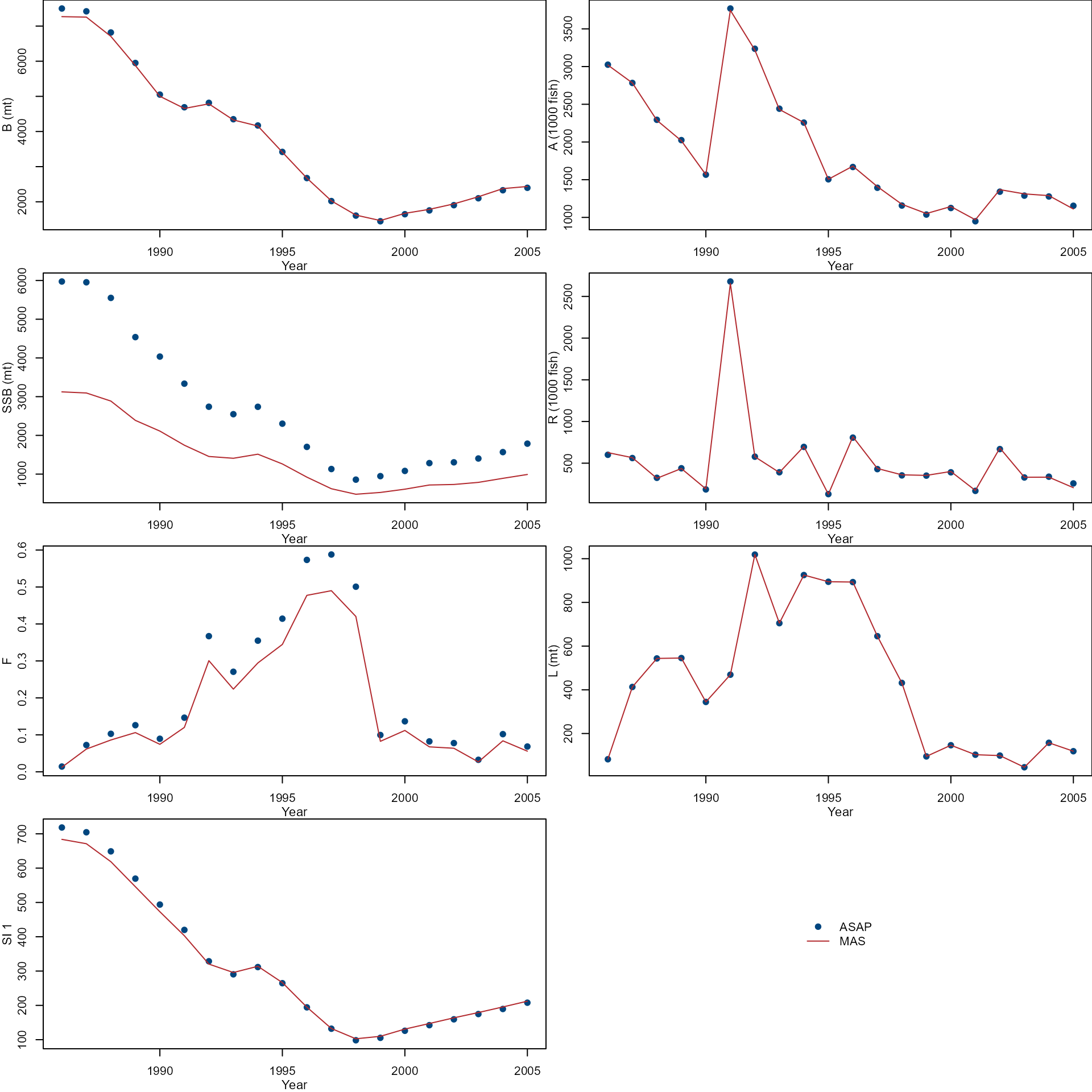
Compare temporal trends of biomass(B), abundance(A), spawning stock biomass (SSB), recruit (R), fishing mortality (F), Landings (L), and Survey index (SI) from ASAP (dots) and MAS (lines).
years <- as.numeric(rownames(asap_output$N.age))
par(mfrow = c(4, 2), mar = c(3, 3, 0, 0))
col <- nmfspalette::nmfs_palette("regional web")(2)
var <- c(
  "biomass", "abundance", "ssb", "recruit", "f",
  "landing", "survey"
)
ylab <- c(
  "B (mt)", "A (1000 fish)",
  "SSB (mt)", "R (1000 fish)",
  "F", "L (mt)", "SI 1"
)
for (i in 1:length(var)) {
  ylim <- range(asap[[var[i]]], mas[[var[i]]])
  plot(years, asap[[var[i]]],
    xlab = "", ylab = "",
    ylim = ylim, pch = 19,
    col = col[1]
  )
  lines(years, mas[[var[i]]],
    col = col[2], lty = 1
  )
  mtext("Year", side = 1, line = 2, cex = 0.7)
  mtext(ylab[i], side = 2, line = 2, cex = 0.7)
}
plot.new()
legend("center",
  c("ASAP", "MAS"),
  pch = c(19, NA),
  lty = c(NA, 1),
  col = col,
  bty = "n"
)
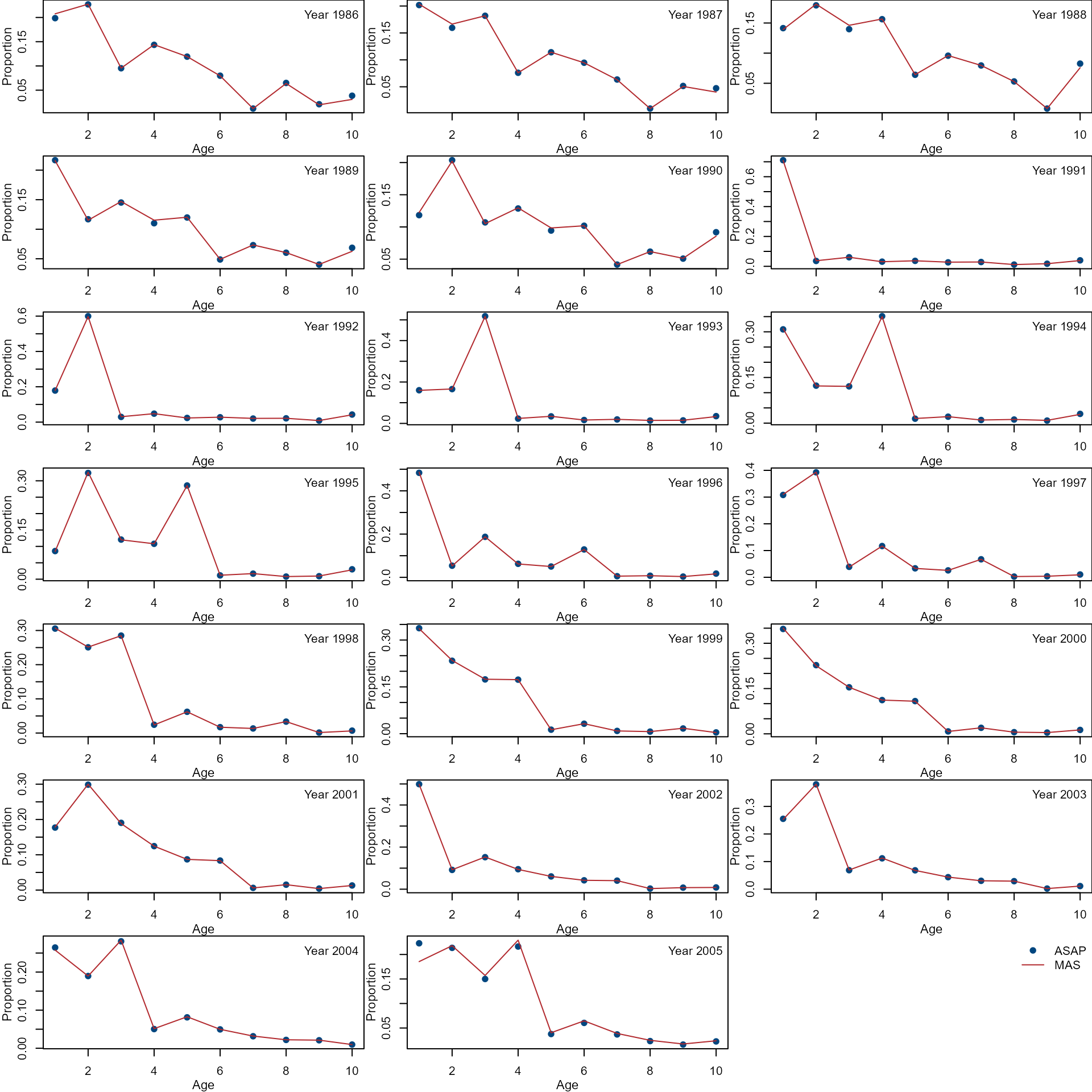
Compare age composition from the ASAP (dots) and MAS (lines).
par(mfrow = c(7, 3), mar = c(3, 3, 0, 0))
col <- nmfspalette::nmfs_palette("regional web")(2)
var <- c("agecomp")
ylab <- c("Proportion")
for (i in 1:ncol(asap[[var]])) {
  ylim <- range(asap[[var]][, i], mas[[var]][, i])
  plot(ages, asap[[var]][, i],
    xlab = "", ylab = "",
    ylim = ylim, pch = 19,
    col = col[1]
  )
  lines(ages, mas[[var]][, i],
    col = col[2], lty = 1
  )
  mtext("Age", side = 1, line = 2, cex = 0.7)
  mtext(ylab, side = 2, line = 2, cex = 0.7)
  legend("topright",
    paste("Year", years[i]),
    bty = "n"
  )
}
plot.new()
legend("topright",
  c("ASAP", "MAS"),
  pch = c(19, NA),
  lty = c(NA, 1),
  col = col,
  bty = "n"
)
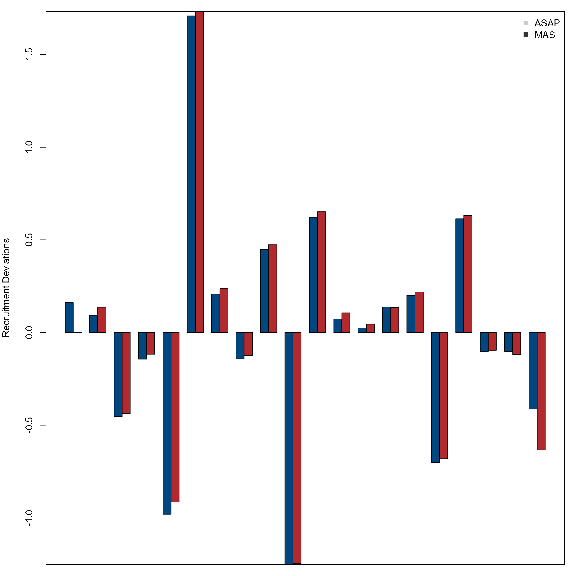
Compare recruitment deviations over years from the OM and MAS.
par(mfrow = c(1, 1), mar = c(1, 4, 1, 1))
col <- nmfspalette::nmfs_palette("regional web")(2)
barplot(rbind(asap$recruit_deviation, mas$recruit_deviation),
  beside = T,
  ylab = "Recruitment Deviations",
  col = col
)
box()
legend("topright",
  c("ASAP", "MAS"),
  col = c("gray80", "gray20"),
  pch = c(15, 15),
  bty = "n"
)
Generate comparison table
Compare estimated R0, q, and h.
# var <- c("R0", "h", "q")
summary_table <- matrix(c(
  asap$r0, mas$r0,
  asap$h, mas$h,
  asap$q, mas$q[[1]]
),
ncol = 2, byrow = TRUE
)
colnames(summary_table) <- c("ASAP", "MAS")
rownames(summary_table) <- c("R0", "h", "q")
summary_table
## ASAP MAS
## R0 471.7017000 456.753108
## h 0.5792984 0.586745
## q 0.1289099 0.116814